
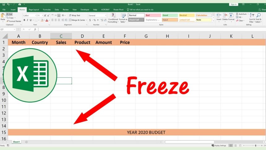
Excel can be both a powerful ally and a bit of a maze—especially when you’re dealing with a huge spreadsheet full of numbers, dates, and text. If you’ve ever scrolled down and forgotten what each column represents, don’t worry. There’s a simple solution: learn how to freeze a row in Excel.
Picture this: You’re working on a spreadsheet with hundreds of rows of data—sales numbers, student scores, budget plans—you name it. As you scroll, your header row disappears, and suddenly you’re guessing what each column stands for. That’s where freezing a row saves the day.
When you know how to freeze a row in Excel, you can lock your headers in place so they stay visible, no matter how far down you scroll. It’s one of those small Excel tricks that can make your work feel much more organized and less stressful.
Why Freezing a Row Helps You Stay on Track
You may think freezing a row is a tiny feature in the grand scheme of Excel. And yes, it’s small—but powerful. Once you start using it, you’ll wonder how you ever worked without it.
Let’s meet Josh, a junior analyst at a logistics company. On his first week on the job, Josh had to review a spreadsheet with more than 3,000 rows. He spent more time scrolling up to check the column labels than he did analyzing the data. Then, a teammate showed him how to freeze a row in Excel, and everything changed. His speed doubled, his accuracy improved, and his stress level dropped instantly.
Josh’s experience isn’t unique. Whether you’re a student, a teacher, a business owner, or just organizing your home expenses, freezing rows can make a big difference in how easily you navigate your data.
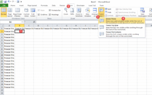
Step-by-Step: How to Freeze a Row in Excel
So how do you actually do it? The good news is, freezing a row is as easy as a few clicks. Here’s how to do it:
Option 1: Freeze the Top Row (Most Common)
This is the option most people use, especially if your headers are in the first row of the spreadsheet.
-
Open your Excel file.
-
Go to the View tab at the top of the window.
-
Click on the Freeze Panes dropdown.
-
Select Freeze Top Row.
Done! Now, even when you scroll down through thousands of rows, your top row stays right where you need it.
Option 2: Freeze Any Specific Row
Maybe your headers aren’t in the first row. Maybe they’re in row 3, 4, or even row 10. No problem—you can freeze any row you like.
-
Click on the row just below the one you want to freeze.
-
For example, if you want to freeze row 5, click on row 6.
-
-
Go to the View tab.
-
Click Freeze Panes > Freeze Panes (yes, the first option again).
Now all the rows above the one you clicked are frozen in place.
Option 3: How to Unfreeze a Row
Changed your mind or made a mistake? No worries. Here’s how to undo it:
-
Go back to the View tab.
-
Click on Freeze Panes.
-
Choose Unfreeze Panes.
That’s all. Everything will go back to normal.
Heading: How to Freeze a Row in Excel Without Overthinking It
A lot of people get nervous about using Excel’s more advanced tools, but freezing rows isn’t one of them. You don’t need formulas, you don’t need programming skills, and you definitely don’t need a degree in data science. You just need to know where to click.
Once you’ve done it a few times, it becomes second nature—just like saving your file or adjusting the font size. It’s one of the easiest ways to make Excel work better for you.
When Should You Freeze a Row?
Freezing rows makes sense in many different situations. Here are just a few:
-
Tracking monthly expenses: Keep the “Month” and “Category” headers visible while scrolling through costs.
-
Sales reports: Lock the client name and invoice columns in place.
-
School projects: Keep assignment titles or grade categories easy to reference.
-
Inventory logs: Maintain product names visible as you browse restock levels.
Basically, anytime you’re dealing with rows of data that rely on headers to make sense, freezing that top row is a smart move.
Bonus Tip: You Can Freeze Rows and Columns
Did you know you can freeze both rows and columns at the same time? This is great for spreadsheets that stretch both down and across.
Here’s how:
-
Click in the cell just below the row and to the right of the column you want to freeze.
-
Go to the View tab.
-
Select Freeze Panes > Freeze Panes.
Now both your row and your column headers will stay in place. Super helpful for large data sets!
Final Thoughts: The Little Feature That Makes Work Feel Easier
When people think about improving productivity, they usually think big—new tools, new systems, complex formulas. But sometimes, it’s the small things that really count. Learning how to freeze a row in Excel is one of those small-but-powerful changes that brings immediate results.
You’ll stop guessing which column you’re in, make fewer mistakes, and save time every time you open your file.
So next time you start a new spreadsheet, take a few seconds to freeze your headers. Your future self will thank you.
Meta Description: Learn how to freeze a row in Excel with this beginner-friendly guide. Keep your headers visible and stay organized while working with large spreadsheets.